Spreadsheets are the engines that run many businesses. With so much data, you will likely have multiple spreadsheets with different information; all of which relate to a single, core piece of your business.  For example, if you are an HR manager, you may have multiple spreadsheets about your employees (one for benefits, one for PTO, one with contact information and one with compensation data). Or, maybe you are a manufacturing company and you have five different spreadsheets with different product details in each.  It can be a chore to consolidate the needed information into a report, prepare a presentation or even just to answer a comprehensive question – unless, of course, you use VLOOKUP!

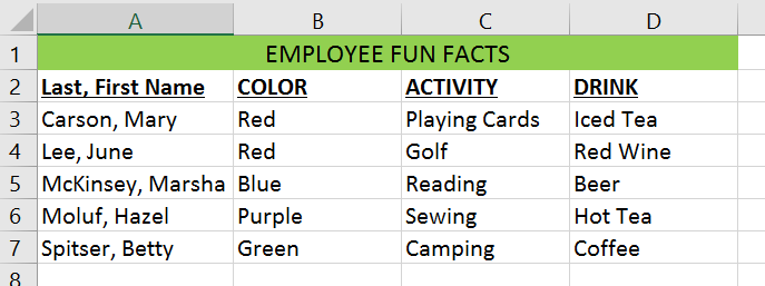
The VLOOKUP function in Excel is one of the most powerful functions out there. Using the HR example above, the following outlines how you can use a VLOOKUP to put together birthday gift baskets for your employees. You have the employee birth date info in one Excel file and their fun facts in another. With more than 500 employees, this would be a tedious task to consolidate manually. But with VLOOKUP, it’s a breeze.

When using VLOOKUPs, you need to have a common data point. This could be a product number, a name, etc.; but it must be unique and common across all data sources you use.  In this case, our common data point will be employee name.  First, you will open both spreadsheets (Employee Fun Facts and Employee Details).

Then, open a new spreadsheet and copy the data from the Employee Details file onto Sheet 2; then copy the data from Employee Fun Facts onto Sheet 3. The first step is to add your common data point to your summary sheet (Sheet 1).  In this case, your common data point is the “Last, First Name” field. You will go to your Employee Details tab and copy the column with “Last, First Name” and paste this to column A on Sheet 1. Now you have a foundation for any data fields you want to pull into your new document. For example, you can pull in the Date of Birth from the Employee Details sheet and then all data fields from the Employee Fun Facts sheet.

Before entering the formulas, it is important to understand the purpose of a VLOOKUP. This formula will look for the common data point you define across multiple sources and will pull back values found in the same rows of anything with that data point as the left-most value in a table.

First, you will add the date of birth. The first column should be the employee names (which you’ve copied and pasted) and then add a second column for “Date of Birth,” which you will pull in using VLOOKUP.

There are four pieces to a VLOOKUP formula. The first is the common data point, this will be the first entry in your formula. In our case, this is found in column A. So, the beginning of the formula is “=vlookup(A3,”  (This is telling your formula that A3 contains that common identifier.)

The next piece of the formula points to where the data lives that you want to pull back into your new sheet.  In this example, we want Excel to go look at Sheet2 (Employee Details), columns A-H, rows 2-7. So the next addition to your formula is “=vlookup(A3,Sheet2!$A$3:$H$7,”.  You can either type this in, or, while you are entering in your formula, simply use the mouse to go click to select the cells on Sheet 2 and then continue your formula.  You will want to hit “F4” after you select the cells as that will make that an absolute reference.  You can also do this by manually adding the “$” sign on the left side of your column and row references. This keeps the reference table static to only those cells.

The first part of the formula tells Excel that you want it to look at Sheet 2 and find that common data point in the table you identified. Next is to tell Excel which column to look for the data on Sheet 2 that you want to pull back to your new sheet. The Date of Birth info is in column F or the 6^th column on Sheet 2. So, now add to your formula: “=VLOOKUP(A3,Sheet2!$A$3:$H$7,6,”.  This tells Excel to pull back the data in the 6^th column that matches your common data point.

The final step of the VLOOKOUP formula is to add a True/False at the end. False indicates the common identifier must be an exact match. True indicates it is an approximate match and is useful when looking for data that falls in a range of values.  You are looking for an exact match, so the equation should read as follows: “=VLOOKUP(A3,Sheet2!$A$3:$H$7,6,FALSE)”. After you enter that formula, drag it down to all rows and you now have the following:

Next you would do the same thing for all the data fields from Sheet 3 Employee Fun Facts. You will want to add VLOOKUP formulas to pull from Sheet 3 columns B, C, and D – a.k.a. columns 2,3 and 4.

The formulas will look as follows:

Color = “=VLOOKUP(A3,Sheet3!$A$2:$D$7,2,FALSE)” – This is pulling the 2^nd column from the 3^rd sheet which is their favorite color.

Activity = “=VLOOKUP(A3,Sheet3!$A$2:$D$7,3,FALSE)” – This is pulling the 3^rd column from the 3^rd sheet which is the employee’s favorite activity.

Drink = “=VLOOKUP(A3,Sheet3!$A$2:$D$7,4,FALSE)” – This is pulling the 4^th column from the 3^rd sheet which is the employee’s favorite drink.

When complete, all of the data will be in one sheet for use!

VLOOKUP can be used to help accomplish various data analysis in any area of your business where data is housed in Excel.

Sandy Noble, Onboarding Controller